How do we interpret the outputs of a neural network trained on classification?
This post shows how neural networks trained for classification approximate the Bayesian posterior, explaining the theoretical basis and providing empirical examples.
This post has been accepted at the ICLR 2025 blogpost track. See the pdf version of this post here.
What do output unit activities really mean?
Deep neural networks trained for classification tasks have been a key driver in the rise of modern deep learning. Training networks for classification is often one of the first lessons or tutorials people encounter when they begin their journey with deep learning. In classification tasks, the multi-class classification problem is one of the most common types of classification problems that people encounter. Widely used datasets, like MNIST, CIFAR-10/100, and ImageNet, are all geared toward the multi-class classification problem. In this problem, the model is trained to receive some data \(X\) as input and infer its class label \(C\) from one of the \(M\) total possible classes. Each data point has one and only one class label from \(M\) possible classes \(c \in \{1 ... M\}\). For example, if we train a convolutional neural network (CNN) to do classification on ImageNet, the data \(X\) is the input image, and the output class label \(C\) is one of the 1000 classes in the ImageNet dataset.
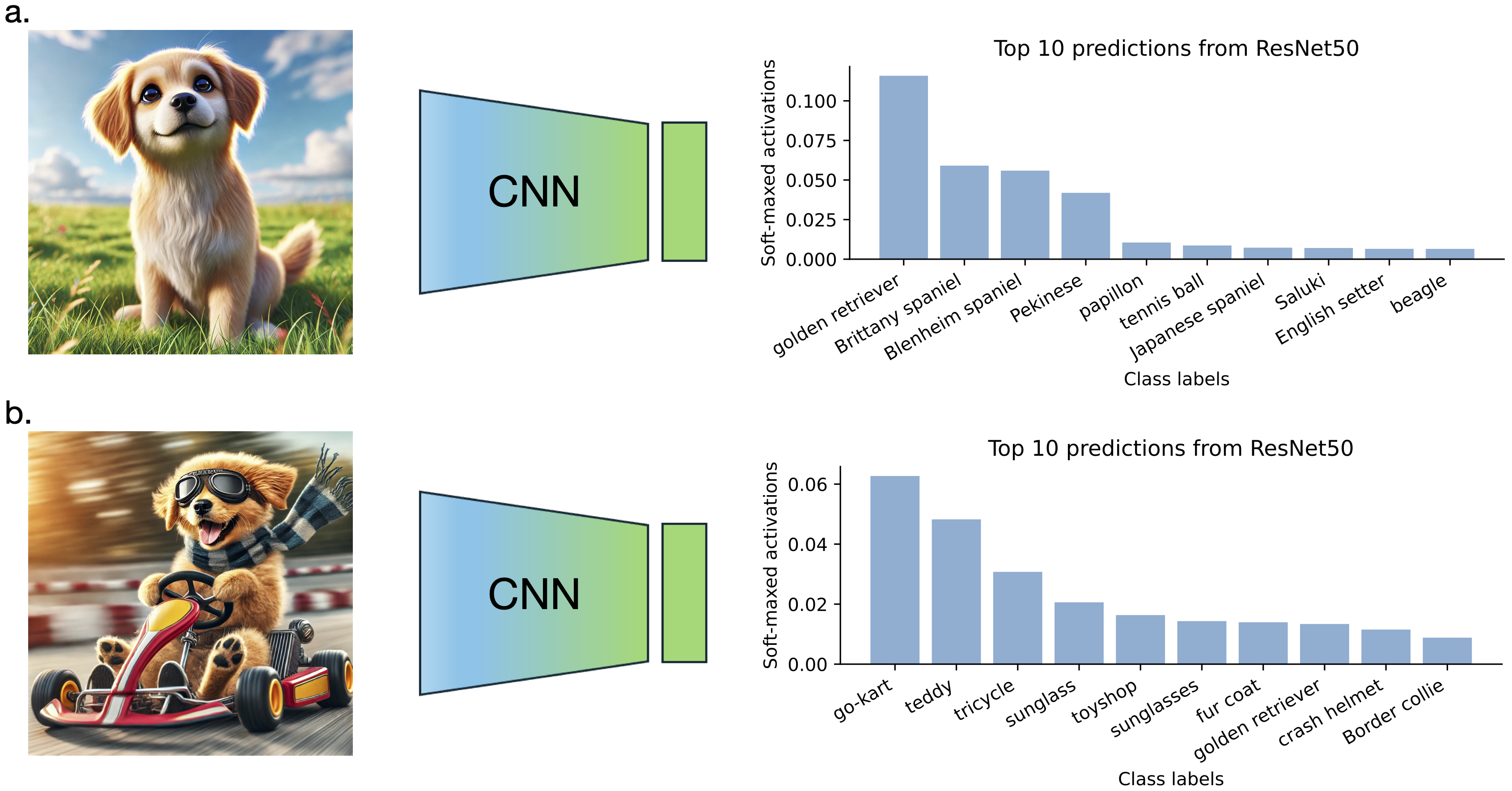
Neural networks trained to do this kind of problem are trained on many input-class label pairs \(\{ (x_j, c_j), j \in 1 ... N \}\) and often have \(M\) output units corresponding to the \(M\) classes in their last layer, called the logit layer. After training the model, most often, people find the unit with the highest value, and its corresponding class is the prediction made by the model. The exact values of activations in the logit layer are often ignored. However, we know that they may be telling us something. For example, if we pass the image in the above figure to a CNN model trained on ImageNet, the best class prediction is “golden retriever.” But the units corresponding to other dog breed categories, like “Brittany spaniel,” “Blenheim spaniel,” “Pekinese,” and “papillon,” also have high activations. The dog breed shown in the image might be ambiguous. In a more complex image of a dog racing a go-kart, the highest output is for the class “go-kart.” However, we also see that the outputs corresponding to “sunglasses,” “golden retriever,” and “crash helmet” have non-negligible activations, reflecting reasonable ambiguity in the true referent of the image.
These examples raise the question: What do the activations in the output layer actually represent? It is commonly understood that after applying the softmax function to the logit layer, the resulting values can be interpreted as probabilities. But what exactly do these probabilities signify? Moreover, how is it that a model trained solely on input-label pairs can represent probabilities across multiple classes?
Here, we try to answer the question: How do we interpret the outputs of a neural network trained on classification? We will show that these probabilities are trained to match the Bayesian posterior probability of an ideal observer having access to a generative model that has generated the data. This also implies that if we have access to the probabilistic generator of the data and class labels, we can train neural network models using input-label pairs to infer the class without performing the often intractable posterior calculation (usually called the “inference” problem).
Previous studies on this topic
Many studies, particularly from the early 1990s, have demonstrated that neural networks can approximate the Bayesian posterior when trained on classification tasks. The mathematical proof and empirical study presented here are inspired by Richard and Lippmann 1991
Deriving the classification objective using maximum likelihood
Before we dive into the interpretation of output activations, let’s first clarify how neural network training is typically set up. For multi-class classification problems, neural networks are commonly designed with \(M\) output units, each corresponding to one of the \(M\) classes. The activations of these output units are passed through a softmax layer, transforming them into a probability distribution over the \(M\) classes, denoted as \(q_{\theta}(C=i \\| X)\), for \(i = 1, \dots, M\). The softmax ensures that each output value lies between 0 and 1, and that the activations of all \(M\) units sum to 1. We denote the activation of the \(i\)-th output unit as \(f_{\theta}^i(X)\), where \(X\) represents the input (e.g., an image), and \(\theta\) represents the trainable parameters of the neural network. After applying the softmax function, the probability assigned to the \(i\)-th class is given by:
\begin{equation} \begin{split} q_{\theta}(C=i|X) = \frac{e^{f_{\theta}^i(X)}}{\sum_{j=1}^M e^{f_{\theta}^j(X)}} \end{split} \end{equation}
The most commonly used loss function for multi-class classification problems can be derived from the maximum likelihood principle. Specifically, we aim to maximize the conditional log-likelihood of the training data under the parameterized model. The training data is represented as \({(x_j, c_j), j = 1, \ldots, N }\), where \(x_j\) is an input (e.g., an image), \(c_j\) is the corresponding class label, and \(N\) is the number of training examples. The resulting loss function, \(\mathbb{L}\), is given below. In practice, if you use PyTorch, this loss function is typically implemented using the cross-entropy loss function. (As we will discuss later, the reason this is called cross-entropy is that the loss function can be understood as the cross-entropy between the model’s predicted output distribution and the empirical distribution of the data.)
\begin{equation} \label{eq:1} \begin{split} \mathbb{L} & = - \frac{1}{N} \sum_{j=1}^N \sum_{i=1}^M \log ({q_{\theta}(C=i|x_j)}) \cdot 1\{c_j = i\}
\end{split} \end{equation}
Here, \(1\{c_j = i\}\) is the indicator function, which takes the value 1 when the class label \(c_j\) equals \(i\), and 0 otherwise. Essentially, for each input, we apply the softmax function over all the output units, then select the unit corresponding to the true class label, take the negative logarithm of that softmax value, and average over all data points. In practice, we optimize this loss function using gradient descent, typically over mini-batches of data, to train the model.
While maximum likelihood is a well-founded approach, it does not directly explain what the output activations represent in a well-trained model when applied to test data. In the following sections, we will show that, a model trained with this objective will be pushed to learn the Bayesian posterior probability over the classes given the data, \(P(C\\|X)\).
Interpretation of outputs as the Bayesian posterior
Minimizing divergence between outputs and the Bayesian posterior
We denote the joint distribution of the input data \(X\), and class labels \(C\) as \(P(X, C)\). The posterior distribution, \(P(C\\|X)\), can be understood as a function that maps the input \(X\) to a probability distribution over the class variable \(C\). Intuitively, computing this posterior aligns with our goal of inferring the probability of each class given the input data. In fact, we will demonstrate that optimizing the network to approximate the posterior \(P(C\\|X)\) is equivalent to training a neural network using the loss function derived in the above section.
We start from the goal of learning the parameters \(\theta\) of a neural network model \(q_{\theta}(C\\|X)\) to approximate the posterior \(P(C\\|X) = \frac{P(X, C)}{P(X)}\). The parameters are learned from the training data \(\{(x_j, c_j), j = 1, \ldots, N \}\). We try to find \(q_\theta\) by minimizing the conditional KL divergence between \(P(C\\|X)\) and \(q_\theta(C\\|X)\):
\begin{equation} \begin{split} \theta^* & = \arg \min_{\theta} \mathbb{L}_{KL}(P(C|X), q_\theta(C|X)) \end{split} \end{equation}
where
\begin{equation} \label{eq:2} \begin{split} \mathbb{L}_{KL}(P(C|X), q_\theta(C|X)) & = \mathbb{E}_{x \sim P(X)} D_{KL}(P(C|x) | q_\theta(C|x)) \end{split} \end{equation}
and we have,
\begin{equation} \begin{split} D_{KL}(P(C|x) | q_\theta(C|x)) & = \mathbb{E}_{c \sim P(C|x)} \log \frac{P(c|x)}{q_\theta(c|x)} \newline & = - H(P(C|x)) - \mathbb{E}_{c \sim P(C|x)} \log q_\theta(c|x) \end{split} \end{equation}
Because \(P\), the ground truth data distribution, does not depend on \(\theta\), the first term in the above equation is fixed. The second term is the cross entropy. So, minimizing \(\mathbb{L}_{KL}(P(C\\|X), q_\theta(C\\|X))\) is equivalent to minimizing the following expected cross-entropy loss:
\begin{equation} \label{eq:3} \begin{split} \mathbb{L}_{CE}(P(C|X), q_\theta(C|X)) & = \mathbb{E}_{x \sim P(X)} \Big[ - \mathbb{E}_{c \sim P(C|x)} \log q_\theta(c|x) \Big] \end{split} \end{equation}
So that,
\begin{equation} \begin{split} \theta^* & = \arg \min_{\theta} \mathbb{L}_{KL}(P(C|X), q_\theta(C|X)) \newline & = \arg \min_{\theta} \mathbb{L}_{CE}(P(C|X), q_\theta(C|X)) \newline & = \arg \min_{\theta} \mathbb{E}_{x \sim P(X)} \Big[ - \mathbb{E}_{c \sim P(C|x)} \log q_\theta(c|x) \Big] \newline & = \arg \min_{\theta} \mathbb{E}_{x \sim P(X)} \Big[ - \int P(c|x) \log q_\theta(c|x) \,dc \Big] \end{split} \end{equation}
In general, to compute the cross-entropy loss, we need to be able to compute the posterior \(P(C\\|X)\). However, in classification problems, we can bypass this by using samples from the joint distribution \((x, c) \sim P(X, C)\). Estimating the loss using samples is tricky, if not impossible, when \(C\) is a continuous variable. However, classification simplifies matters because class label \(C\) is a discrete random variable that takes a finite set of possible values \(c \in \{1, ..., M\}\). So, we can write the loss function as:
\begin{equation} \begin{split} \mathbb{L}_{CE}(P(C|X), q_\theta(C|X)) & = \mathbb{E}_{x \sim P(X)} \Big[ - \sum_{i=1}^M P(C=i|x) \log q_\theta(C=i|x) \Big] \end{split} \end{equation}
It is possible to derive a loss function \(\overline{\mathbb{L}}_{CE}(P(C\\|X), q_\theta(C\\|X))\) that achieve the same objective as \(\mathbb{L}_{CE}(P(C\\|X), q_\theta(C\\|X))\) when being minimized. We can instead optimize the following empirical cross-entropy loss:
\begin{equation} \label{eq:4} \begin{split} \overline{\mathbb{L}}_{CE}(P(C|X), q_\theta(C|X)) & = \mathbb{E}_{(x,c) \sim P(X,C)} \Big[ - \sum_{i=1}^M \log ({q_{\theta}(C=i|x)}) \cdot 1\{c = i\} \Big] \end{split} \end{equation}
The indicator function \(1\{c = i\}\) takes the value 1 only when the class label for a given data sample is \(c = i\), and 0 otherwise. We can show that \(\overline{\mathbb{L}}_{CE}(P(C\\|X), q_\theta(C\\|X))\) is the same as the cross entropy loss \(\mathbb{L}_{CE}(P(C\\|X), q_\theta(C\\|X))\)
\begin{equation} \begin{split} \overline{\mathbb{L}}_{CE}(P(C|X), q_\theta(C|X)) & = \mathbb{E}_{(x,c) \sim P(X,C)} \Big[ - \sum_{i=1}^M \log ({q_{\theta}(C=i|x)}) \cdot 1\{c = i\} \Big] \newline & = - \mathbb{E}_{x \sim P(X)} \Big[ \mathbb{E}_{c \sim P(C|x)} \Big[ \sum_{i=1}^M \log ({q_{\theta}(C=i|x)}) \cdot 1\{c = i\} \Big] \Big] \newline & = - \mathbb{E}_{x \sim P(X)} \Big[ \sum_{i=1}^M P(C=i|x) \log ({q_{\theta}(C=i|x)}) \Big] \newline & = \mathbb{L}_{CE}(P(C|X), q_\theta(C|X)) \end{split} \end{equation}
In summary, we have shown that minimizing \(\overline{\mathbb{L}}_{CE}(P(C\\|X), q_\theta(C\\|X))\) is equivalent to minimizing \(\mathbb{L}_{CE}(P(C\\|X), q_\theta(C\\|X))\), which in turn is equivalent to minimizing \(\mathbb{L}_{KL}(P(C\\|X), q_\theta(C\\|X))\), the conditional KL divergence between \(P(C\\|X)\) and \(q_\theta(C\\|X)\).
In practice, the loss is estimated by taking mini-batches of data \(\{(x_j, c_j), j = 1, ..., N\}\) and we use stochastic gradient descent to find \(\theta^*\) by minimizing the following loss:
\begin{equation} \begin{split} \overline{\mathbb{L}}_{CE}(P(C|X), q_\theta(C|X)) & \approx \widehat{\mathbb{L}}_{CE}(P(C|X), q_\theta(C|X)) \newline & = - \frac{1}{N} \sum_{j=1}^N \sum_{i=1}^M \log ({q_{\theta}(C=i|x_j)}) \cdot 1\{c_j = i\} \end{split} \end{equation}
This objective is identical to the one derived from the maximum likelihood principle in Equation \eqref{eq:1}. In summary, we have shown that minimizing the objective derived from maximum likelihood (Equation \eqref{eq:1}) is equivalent to minimizing the conditional KL divergence between the model’s output and the Bayesian posterior (Equation \eqref{eq:2}).
Loss is minimized when outputs exactly match the posterior
When is the loss minimized? We can answer this question through deriving a lower bound of the objective function \(\overline{\mathbb{L}}_{CE}(P(C\\|X), q_\theta(C\\|X))\).
\begin{equation} \begin{split} \overline{\mathbb{L}}_{CE}(P(C|X), q_\theta(C|X)) & = - \mathbb{E}_{x \sim P(X)} \Big[ \sum_{i=1}^M P(C=i|x) \log ({q_{\theta}(C=i|x)}) \Big] \newline & \geq - \mathbb{E}_{x \sim P(X)} \Big[ \sum_{i=1}^M P(C=i|x) \log ({P(C=i|x)}) \Big] \end{split} \end{equation}
In the final step, we apply Gibbs’ inequality. For \(x \sim P(X)\), the loss \(\overline{\mathbb{L}}_{CE}(P(C\\|X), q_\theta(C\\|X))\) is minimized when the bound becomes tight, which occurs when:
\begin{equation} \begin{split} q_{\theta^*}(C=i|x) = P(C=i|x), \quad i \in \{1, …, M\} \end{split} \end{equation}
The loss is minimized when the model’s outputs exactly matches the Bayesian posterior.
How to interpret the network outputs
Let us return to our original question: What do the activations in the output layer actually represent? Our analysis has shown that the softmax output activations are trained to approximate the Bayesian posterior as closely as possible. The Bayesian posterior is computed under the assumption that there is a generative model \(P(X, C)\) that has produced the data, and Bayes’ rule is applied: \(P(C\\|X) = \frac{P(X, C)}{P(X)}\) to calculate the posterior.
In most real-world tasks, such as ImageNet classification, we do not have access to the true generative model of the data, making it impossible to compute the exact posterior. So, the interpretation of the output unit activities is a hypothetical one: The soft-maxed outputs approximate the Bayesian posterior calculated using a generative model of the data, if someone can find such a model. However, in some cases, we have access to the generative model. Our results imply that the soft-maxed output activities of the networks will approximate the Bayesian posterior calculated theoretically using the generative model. We will explore this further with specific examples in the following section.
Empirical studies with known generative models
A simple classification example
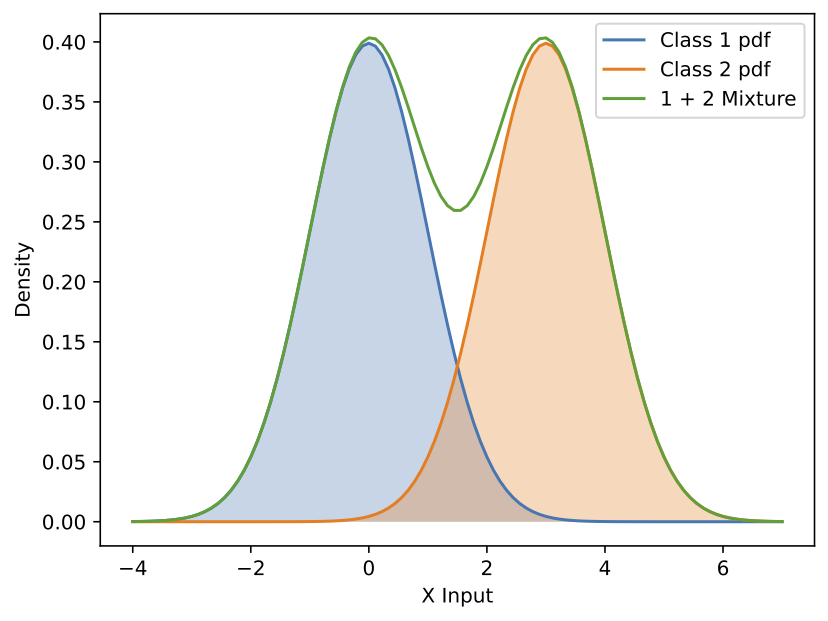
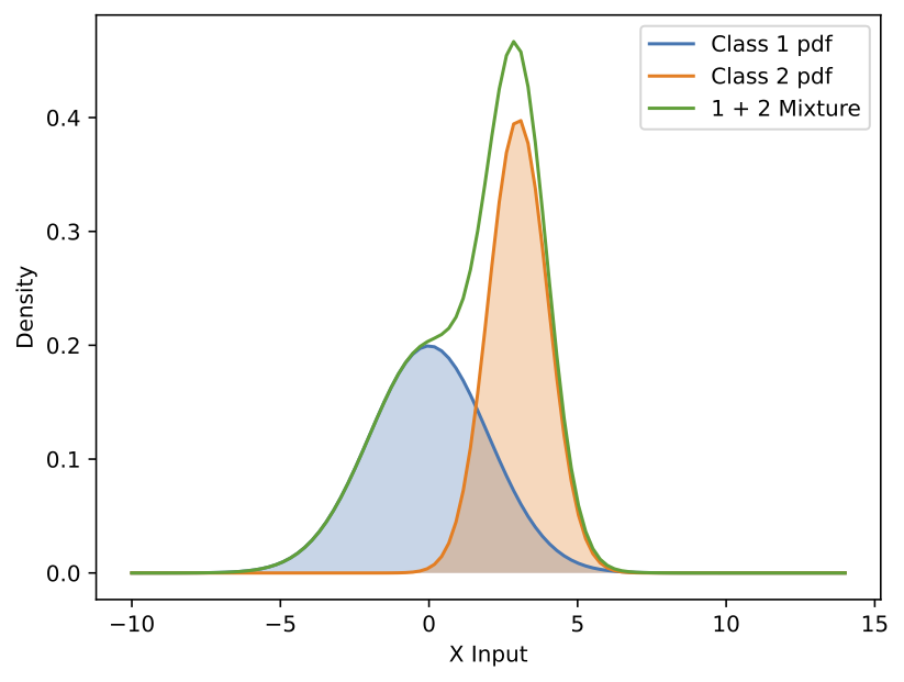
Now, let us explore a basic empirical example. Suppose we observe a single data point, \(x\), which is drawn from one of two possible classes, \(C = c_1\) or \(C = c_2\), with equal prior probabilities, i.e., \(P(c_1) = P(c_2) = 0.5\). Once the class is determined, the probability distribution of \(x\) given each class follows a Gaussian distribution, as shown in the figure below.
\begin{equation} \begin{split} P(x|c_1) = \frac{1}{\sqrt{2 \pi \sigma_1^2} } e^{-\frac{(x-\mu_1)^2}{2\sigma_1^2}} \text{, where} \, \sigma_1=1 \text{, } \mu_1=0 \newline P(x|c_2) = \frac{1}{\sqrt{2 \pi \sigma_2^2} } e^{-\frac{(x-\mu_2)^2}{2\sigma_2^2}} \text{, where} \, \sigma_2=1 \text{, } \mu_2=3 \end{split} \end{equation}
When we observe a new data point \(x\), we want to infer which class it belongs to. Intuitively, in the example above, if \(x\) is small, it is more likely to belong to the first class, while if \(x\) is large, it is more likely to belong to the second class. Concretely, there are two ways we can approach this problem:
1. Train neural networks with input-label pairs. One approach is to train a neural network using a dataset of many labeled examples, represented as pairs \({(x_j, c_j), j = 1 \dots N }\). We can train a neural network model that takes \(x\) as input and predicts the corresponding class, optimizing the loss function in Equation \eqref{eq:1}. This method allows us to infer the class of new data without knowing the underlying generative process. The code to do the above is posted here: https://github.com/YudiXie/interpret-classification
2. Derive the Bayesian posterior theoretically. Another way to solve this problem is to derive it theoretically using Bayes’ rule. Given \(x\), the posterior probability of \(x\) has class label \(c_1\) or \(c_2\) can be computed using Bayes’ rule:
\begin{equation} \begin{split} P(c_1|x) & = \frac{P(x|c_1) P(c_1)}{P(x)} = \frac{P(x|c_1) P(c_1)}{P(x|c_1) P(c_1) + P(x|c_2) P(c_2)} \newline & = \frac{1}{1 + \frac{\sigma_1}{\sigma_2} e^{\frac{\sigma_2^2(x-\mu_1)^2 - \sigma_1^2(x-\mu_2)^2}{2 \sigma_1^2 \sigma_2^2}}} \newline & = \frac{1}{1 + e^{\frac{6x-9}{2}}} \end{split} \end{equation}
\begin{equation} \begin{split} P(c_2|x) & = \frac{P(x|c_2) P(c_2)}{P(x)} = \frac{P(x|c_2) P(c_2)}{P(x|c_1) P(c_1) + P(x|c_2) P(c_2)} \newline & = \frac{1}{1 + \frac{\sigma_2}{\sigma_1} e^{\frac{\sigma_1^2(x-\mu_2)^2 - \sigma_2^2(x-\mu_1)^2}{2 \sigma_1^2 \sigma_2^2}}} \newline & = \frac{1}{1 + e^{\frac{-6x+9}{2}}} \end{split} \end{equation}
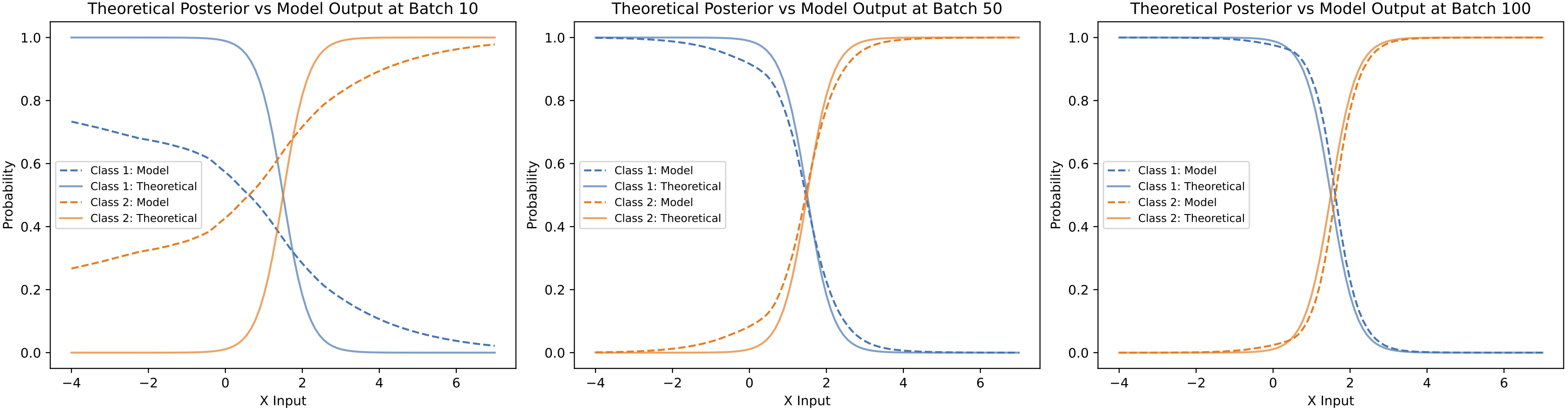
In the previous section, we proved that the theoretically derived Bayesian posterior is the solution that minimizes the loss function used to train the neural network. But, do networks actually learn the Bayesian posterior empirically? The above figure compares the theoretical solution with the solution learned by the neural network at different stages of training. As shown, the model gradually approximates the theoretical solution over the course of mini-batch updates. After 100 batches, the model’s output is nearly identical to the theoretical solution.
A harder example with a more complex posterior
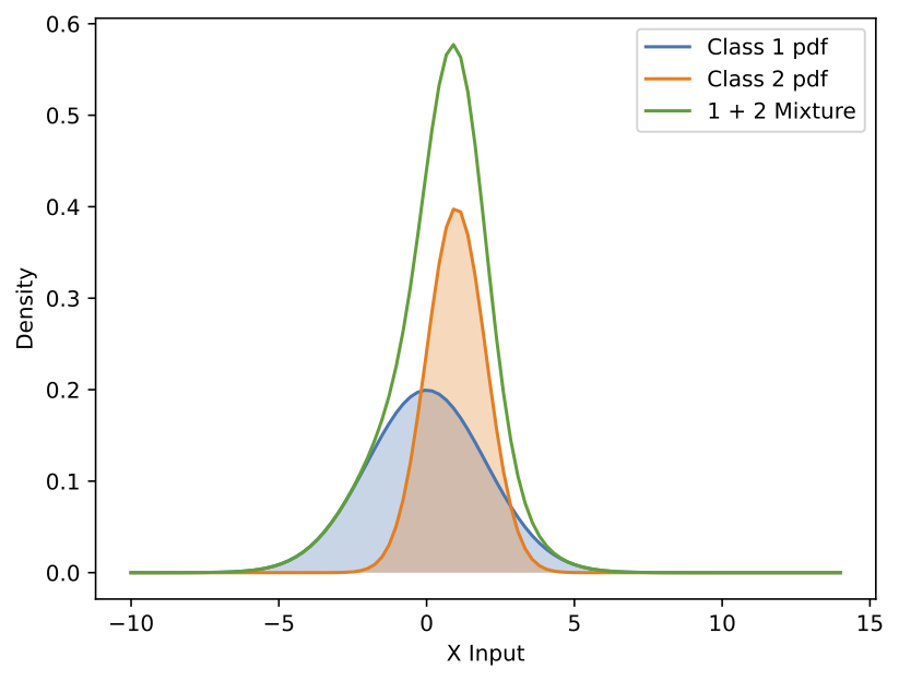
Let us see another example in the above figure when \(\sigma_1=2 \text{, } \mu_1=0\) and \(\sigma_2=1 \text{, } \mu_2=1\). The posterior distribution is more complex in this case than in the previous example. As we move along the x-axis from left to right, \(P(C=c_1\\|x)\) initially dominates over \(P(C=c_2\\|x)\), but this reverses when \(x\) becomes greater than roughly 0. Interestingly, for \(x\) values larger than around 3, \(P(C=c_1\\|x)\) once again surpasses \(P(C=c_2\\|x)\) because the probability density of class 2 drops faster than that of class 1. Can a neural network capture this more complex posterior after training?
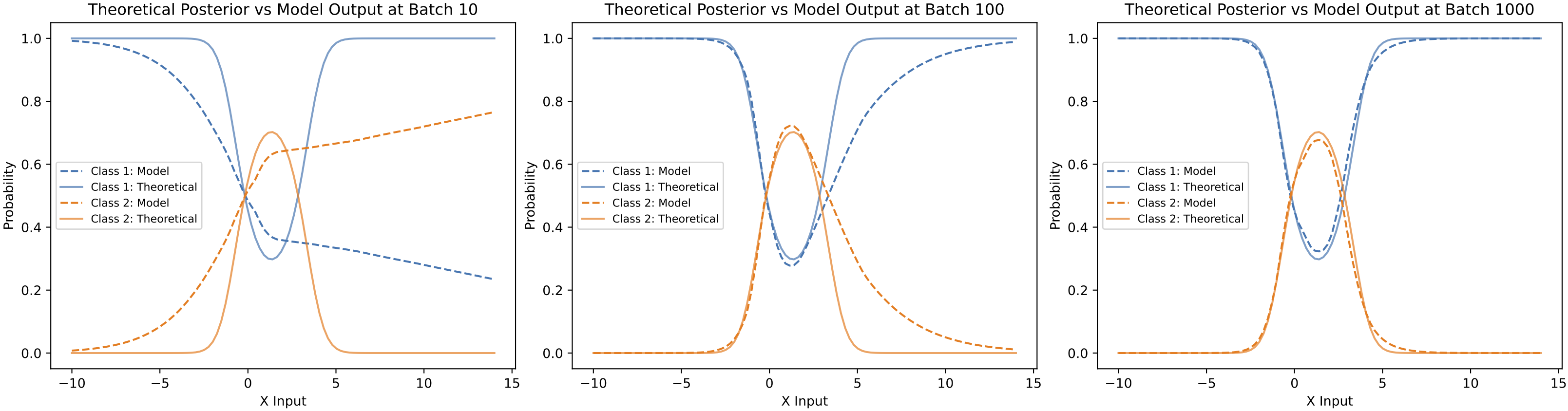
In the above figure, we compare the theoretically derived Bayesian posterior with the neural network output at different stages of training. Like the previous example, the network gradually approximates the posterior shape during training. However, unlike the earlier case, the network requires more training examples to approximate this more complex posterior accurately. Noticeable gaps remain between the model’s output and the theoretical result at 100 batches, and only after 1000 mini-batch updates does the network achieve a reasonably accurate approximation of the posterior.
An even harder classification example
Let us consider an even more challenging example, shown in the above figure, where we set \(\sigma_1=2\), \(\mu_1=0\), and \(\sigma_2=1\), \(\mu_2=3\). Compared to the previous example, the only change is that the center of the class 2 distribution has been shifted to the right. While the shape of the theoretically derived posterior remains quite similar to the earlier case, this shift makes it even more difficult for the model to learn the posterior accurately.
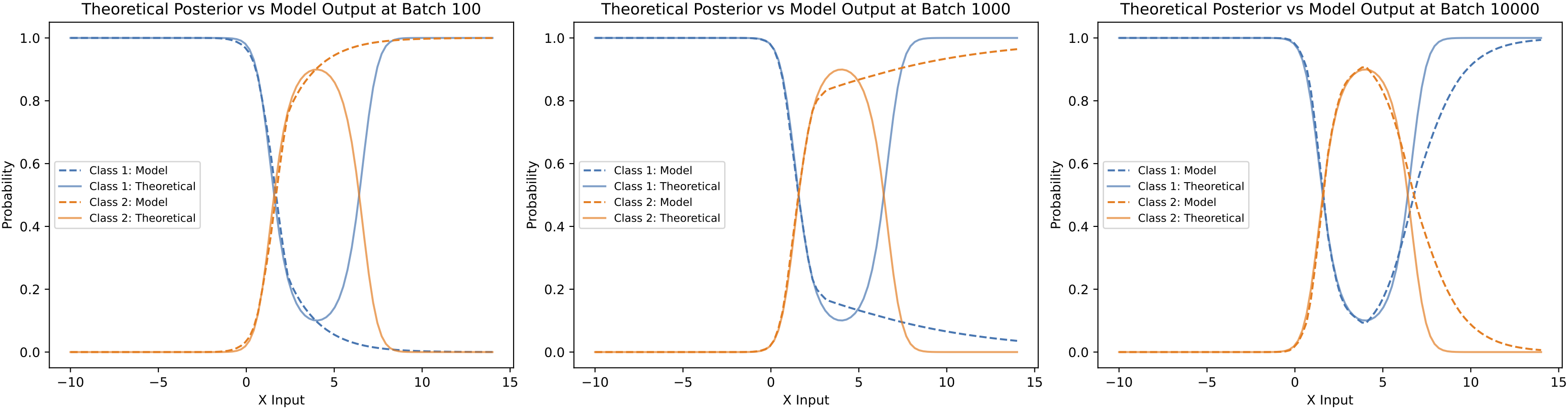
As shown in the above figure, after 1000 mini-batch updates, the model successfully learns the first crossing point of the posterior on the left, but it struggles to capture the second crossing point. Even after 10,000 batches, the model’s output still deviates significantly from the theoretical posterior. One potential reason for this difficulty is that very little probability mass is concentrated on the right side of the x-axis for both classes. The sparsity of the training data in that region makes it much harder for the model to learn the posterior shape correctly.
In summary, we have shown that the model approximates the posterior well in many simple cases. However, the model’s ability to accurately approximate the posterior depends not only on the complexity of the shape of the posterior, but also on the underlying data distribution. In regions where the data is sparse, it becomes much more challenging for the model to learn the correct posterior shape.
Conclusions and discussions
In this tutorial, we explored how to interpret the output activations of neural networks trained on classification tasks. Through theoretical derivations, we demonstrated that these activations, after applying the softmax function, should closely approximate the Bayesian posterior probabilities. Specifically, minimizing the cross-entropy loss function commonly used in classification is equivalent to minimizing the conditional KL divergence between the network’s outputs and the Bayesian posterior, and the loss is minimized when the network outputs exactly match the Bayesian posterior.
Our empirical studies illustrated that neural networks indeed approximate the posterior well in simpler classification scenarios. However, as the complexity of the posterior increases or as data becomes sparse in certain regions, accurate approximation becomes significantly more challenging. These findings emphasize that while neural network outputs can be interpreted as the approximation to the Bayesian posterior, the quality of the approximation depends heavily on factors such as posterior complexity and data availability. The approximation quality will also depends on the network architecture and optimization details, which we did not explore here.
It is worth noting that the theoretical derivation we presented here only applies to classification tasks where the output is a discrete random variable that takes a finite set of values. The interpretation of network outputs in other cases, such as regression tasks, will depends on the specific formulations.
We hope that clarifying the interpretation of classification network outputs encourages us to view them not just as simple predictions, but as rich probabilistic representations that reflect uncertainty and ambiguity inherent in the data.
If you spot any mistakes or errors in this post, feel free to leave a comment below or reach out to me via the email provided on the main page. I’d be happy to correct them promptly 😊
If you found this useful, you can cite this as:
@inproceedings{xie2025we,
  title={How do we interpret the outputs of a neural network trained on classification?},
  author={Xie, Yudi},
  booktitle={The Fourth Blogpost Track at ICLR 2025},
  year={2025},
}